Deep Learning
post on 26 Dec 2019 about 8233words require 28min
CC BY 4.0 (除特别声明或转载文章外)
如果这些文字帮助到你,可以请我喝一杯咖啡~
Convolutional Neural Networks (CNNs / ConvNets)
- Chinese version: https://www.zybuluo.com/hanbingtao/note/485480
- English version: http://cs231n.github.io/convolutional-networks/#layers
Architecture Overview
Regular Neural Nets don’t scale well to full images. In CIFAR-10, images are only of size $32\times 32\times 3$ (32 wide, 32 high, 3 color channels), so a single fully-connected neuron in a first hidden layer of a regular Neural Network would have $32323$ = 3072 weights. This amount still seems manageable, but clearly this fully-connected structure does not scale to larger images. For example, an image of more respectable size, e.g. $200\times 200\times 3$, would lead to neurons that have 200*200*3 = 120,000 weights. Moreover, we would almost certainly want to have several such neurons, so the parameters would add up quickly! Clearly, this full connectivity is wasteful and the huge number of parameters would quickly lead to overfitting.
Convolutional Neural Networks take advantage of the fact that the input consists of images and they constrain the architecture in a more sensible way. In particular, unlike a regular Neural Network, the layers of a ConvNet have neurons arranged in 3 dimensions: width, height, depth. (Note that the word depth here refers to the third dimension of an activation volume, not to the depth of a full Neural Network, which can refer to the total number of layers in a network.) For example, the input images in CIFAR-10 are an input volume of activations, and the volume has dimensions $32\times 32\times 3$ (width, height, depth respectively). As we will soon see, the neurons in a layer will only be connected to a small region of the layer before it, instead of all of the neurons in a fully-connected manner. Moreover, the final output layer would for CIFAR-10 have dimensions $1\times 1\times 10$, because by the end of the ConvNet architecture we will reduce the full image into a single vector of class scores, arranged along the depth dimension. Here is a visualization:
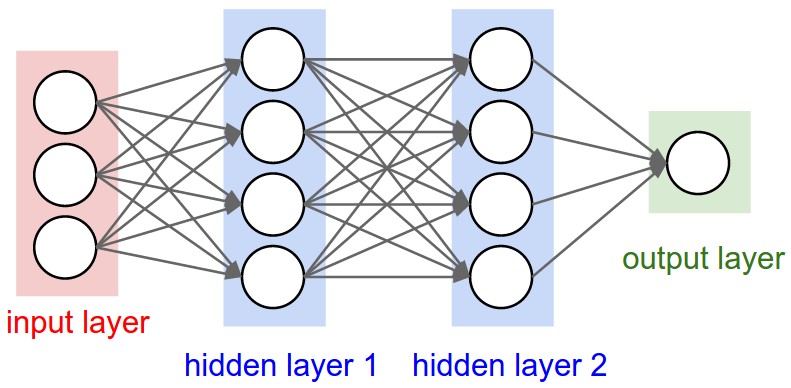
A regular 3-layer Neural Network
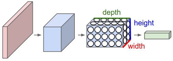
A ConvNet arranges its neurons in three dimensions (width, height, depth), as visualized in one of the layers. Every layer of a ConvNet transforms the 3D input volume to a 3D output volume of neuron activations. In this example, the red input layer holds the image, so its width and height would be the dimensions of the image, and the depth would be 3 (Red, Green, Blue channels)
Layers used to build ConvNets
A simple ConvNet is a sequence of layers, and every layer of a ConvNet transforms one volume of activations to another through a differentiable function. We use three main types of layers to build ConvNet architectures: Convolutional Layer, Pooling Layer, and Fully-Connected Layer (exactly as seen in regular Neural Networks). We will stack these layers to form a full ConvNet architecture.

Example Architecture: Overview. We will go into more details below, but a simple ConvNet for CIFAR-10 classification could have the architecture [INPUT - CONV - RELU - POOL - FC]. In more detail:
- INPUT [$32\times 32\times 3$] will hold the raw pixel values of the image, in this case an image of width 32, height 32, and with three color channels R,G,B.
- CONV layer will compute the output of neurons that are connected to local regions in the input, each computing a dot product between their weights and a small region they are connected to in the input volume. This may result in volume such as [$32\times 32\times 12$] if we decided to use 12 filters.
- RELU layer will apply an elementwise activation function, such as the $max(0,x)$ thresholding at zero. This leaves the size of the volume unchanged ([$32\times 32\times 12$]).
- POOL layer will perform a downsampling operation along the spatial dimensions (width, height), resulting in volume such as [$16\times 16\times 12$].
- FC (i.e. fully-connected) layer will compute the class scores, resulting in volume of size [$1\times 1\times 10$], where each of the 10 numbers correspond to a class score, such as among the 10 tags of CIFAR-10. As with ordinary Neural Networks and as the name implies, each neuron in this layer will be connected to all the numbers in the previous volume.
Convolutional Layer
To summarize, the Conv Layer:
- Accepts a volume of size $W_1\times H_1\times D_1$
- Requires four hyperparameters:
- Number of filters $K$,
- their spatial extent $F$,
- the stride $S$,
- the amount of zero padding $P$.
- Produces a volume of size $W_2\times H_2\times D_2$ where:
- $W_2=(W_1-F+2P)/S+1$
- $H_2=(H_1-F+2P)/S+1$ (i.e. width and height are computed equally by symmetry)
- $D_2=K$
- With parameter sharing, it introduces $F\cdot F\cdot D_1$ weights per filter, for a total of $(F\cdot F\cdot D_1)\cdot K$ weights and $K$ biases.
- In the output volume, the $d$-th depth slice (of size $W_2\times H_2$) is the result of performing a valid convolution of the $d$-th filter over the input volume with a stride of $S$, and then offset by $d$-th bias.
A common setting of the hyperparameters is $F=3$,$S=1$,$P=1$. However, there are common conventions and rules of thumb that motivate these hyperparameters.


Pooling Layer
It is common to periodically insert a Pooling layer in-between successive Conv layers in a ConvNet architecture. Its function is to progressively reduce the spatial size of the representation to reduce the amount of parameters and computation in the network, and hence to also control overfitting. The Pooling Layer operates independently on every depth slice of the input and resizes it spatially, using the \textbf{MAX} operation. The most common form is a pooling layer with filters of size $2\times 2$ applied with a stride of 2 downsamples every depth slice in the input by 2 along both width and height, discarding $75\%$ of the activations. Every MAX operation would in this case be taking a max over 4 numbers (little $2\times 2$ region in some depth slice). The depth dimension remains unchanged. More generally, the pooling layer:
- Accepts a volume of size $W_1\times H_1\times D_1$
- Requires two hyperparameters:
- their spatial extent $F$,
- the stride $S$,
- Produces a volume of size $W_2\times H_2\times D_2$ where:
- $W_2=(W_1-F)/S+1$
- $H_2=(H_1-F)/S+1$
- $D2=D1$
- Introduces zero parameters since it computes a fixed function of the input
- For Pooling layers, it is not common to pad the input using zero-padding.
The CIFAR-10 dataset
The CIFAR-10 dataset (http://www.cs.toronto.edu/~kriz/cifar.html) consists of 60000 $32\times 32$ colour images in 10 classes, with 6000 images per class. There are 50000 training images and 10000 test images.
The dataset is divided into five training batches and one test batch, each with 10000 images. The test batch contains exactly 1000 randomly-selected images from each class. The training batches contain the remaining images in random order, but some training batches may contain more images from one class than another. Between them, the training batches contain exactly 5000 images from each class. Here are the classes in the dataset, as well as 10 random images from each:

The classes are completely mutually exclusive. There is no overlap between automobiles and trucks. “Automobile” includes sedans, SUVs, things of that sort. “Truck” includes only big trucks. Neither includes pickup trucks.
Tasks
- Given the data set in the first section, please implement a convolutional neural network to calculate the accuracy rate. The major steps involved are as follows:
- Reading the input image.
- Preparing filters.
- Conv layer: Convolving each filter with the input image.
- ReLU layer: Applying ReLU activation function on the feature maps (output of conv layer).
- Max Pooling layer: Applying the pooling operation on the output of ReLU layer.
- Stacking conv, ReLU, and max pooling layers
- You can refer to the codes in cs231n. Don’t use Keras, TensorFlow, PyTorch, Theano, Caffe, and other deep learning softwares.
Codes and Results
在终端中执行下述指令,获取 cs231n 的数据集并本地编译。
1
2
3
4
cd cs231n/datasets
./get_datasets.sh
cd ../
python setup.py build_ext --inplace
回到初始目录,执行下属指令进行学习,并将日志写入screen.log。(CPU 上跑了快一个小时…)
1
python main.py | tee screen.log
训练了 10 个 Epoch 共 4900 次迭代,最后得到的结果如下(screen.log),在训练集上得到了大约百分之七十的准确度。
1
(Epoch 10 / 10) train acc: 0.706000; val_acc: 0.598000
运行结果过程中的 Loss 函数变化如下图。

main.py
所需要实现的部分已经在cs231n中有了,这里只用import进来进行训练即可。这里使用了默认的参数进行训练,已经得到了比较不错的结果。
1
2
3
4
5
6
7
8
9
10
11
from cs231n.data_utils import get_CIFAR10_data
from cs231n.classifiers.cnn import ThreeLayerConvNet
from cs231n.solver import Solver
from matplotlib import pyplot
if __name__ == '__main__':
    solver = Solver(ThreeLayerConvNet(), get_CIFAR10_data())
    solver.train()
    pyplot.plot(solver.loss_history)
    pyplot.xlabel("Iteration")
    pyplot.ylabel("Loss")
    pyplot.show()
Reflection
由于临近期末,本次实验没有假如像之前 BP 算法和神经网络一样完全手写,而是参考了来自 cs231n 的代码,剩下的核心任务就是编写 main 函数来训练 CNN 了。其中使用到的 CNN 示意图大致如下。
和全连接网络相比,卷积神经网络使用了局部连接(每个神经元之和上一层的少数而非全部神经元连接)、权值共享(一组连接共享同一个权重)、下采样(增加一个池化的步骤提取样本特征)三个方面的方法,通过尽可能保留重要的参数(利用样本数据的特征,例如图像识别中相邻像素关系紧密),去掉大量不重要的参数,来达到更好的学习效果。
和全连接神经网络相比,卷积神经网络的训练要复杂一些。但训练的原理是一样的:利用链式求导计算损失函数对每个权重的偏导数(梯度),然后根据梯度下降公式更新权重。训练算法依然是反向传播算法,详细的公式推导在前面的作业引导中已经有了。
由于不可以使用常见的深度学习框架,这次大量的计算在 CPU 上跑了将近一个小时…做机器学习是真的吃计算资源。想来近些年深度学习能够如此火热的原因很大一部分也要归功于算力的发展吧。
话说回来,一个学期的实验课终于到此结束。回看这一学期,一共做了 16 个 Lab、4 个 Project、4 个 Theory、1 个 Presentation(因为没有经验被老师怼的很惨)。总的来说,我觉得这门人工智能是我这个学期知识容量最大的一门课,也确实让人学到了很多知识(我奇怪于这门课在前一个年级是必修课,但是在今年却变成了选修)。从最开始的搜索(宽搜、迭代加深搜索、对抗搜索以及最小最大剪枝等等),再之后的知识表达(Prolog、Strips),最后到机器学习,课程和实验的难度都在不断提升,每个礼拜都要花掉好几整天的时间在这门课上,远远超出了 TA 说的「实验内容都可以在课上完成」,可能还是我太菜了吧。尤其是最后的机器学习部分,写代码的过程中伴随着大量的公式推导,让人感叹自己数学直觉和功底的差劲。不过,这门课的设计还是非常棒的,各种作业的背景也很有趣且有用。希望这门课上学到的知识能够在以后真正的派上用场~
Related posts